TIPS FOR SUCCESSFUL DE NOVO TRANSCRIPTOME SEQUENCE ASSEMBLY
USING RNA-SEQ DATA
DOWNLOAD THIS GUIDE
Home > Product Literature > Contaminant Removal and Transcriptome Annotation | DNASTAR
Chapter 2: Using Lasergene Genomics to Streamline the Workflow
Using Lasergene Genomics to streamline the workflow
Three applications in the Lasergene Genomics package—SeqMan NGen, SeqMan Ultra, and ArrayStar— work together as an integrated pipeline for de novo transcriptome assembly and downstream analysis.
Remove contaminants and assemble and annotate the transcripts
SeqMan NGen is an all-in-one tool for removing adapter and other contaminants, assembling the transcripts, and then automatically annotating them with group-specific annotations. This tool requires only 1-2 minutes of hands-on time to set up the assembly, and covers “Software Steps 1-3” from the previous section of this ebook.
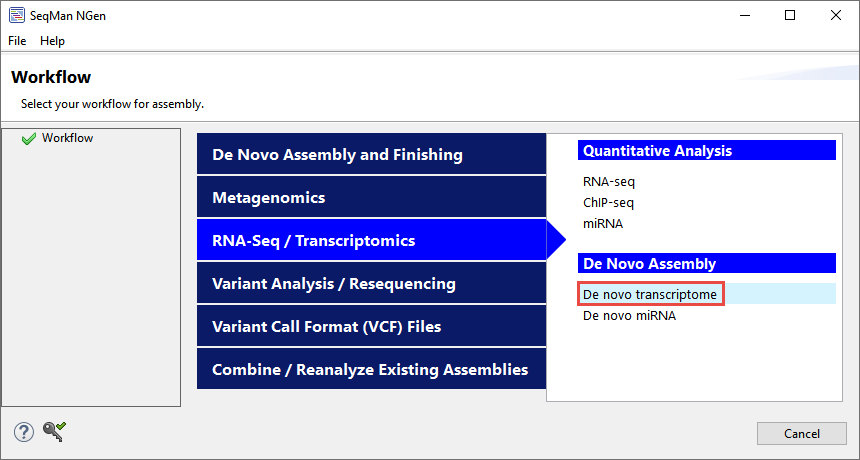
To set up the assembly, launch SeqMan NGen and choose the “De novo transcriptome” workflow (Figure 3).

Figure 3. Selecting the workflow in the SeqMan NGen wizard.
After that, follow the prompts to specify automatic removal of the most common adapters, including Illumina Universal Adapter, as well as any rRNA contaminant sequences or vectors that you specify (Figures 2 and 4).

Figure 4. SeqMan NGen lets you screen for specific rRNA contaminants by checking a box and adding one or more contaminant files.
You then upload your de novo transcriptome reads.
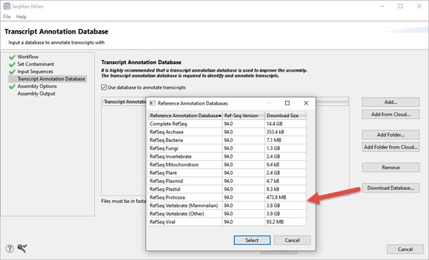
During setup, be sure to check the box (Figure 5) to automatically annotate transcripts using DNASTAR’s proprietary Transcript Annotation Database.

Figure 5. Selecting the desired Transcript Annotation Database in the SeqMan NGen wizard.
Click the Download Database button and select an mRNA database from related taxa or select the entire RefSeq database. These databases are sets of reference mRNAs that include both sequence data and transcript annotations extracted from data on NCBI’s RefSeq website. Because you are selecting from a broad biological group, rather than a single species, these annotations can be used to facilitate assembly and annotation both model and non-model organisms from over a dozen organism groups. (Note: If you don’t have Internet access in your lab, you can alternatively use a local copy of RefSeq as the annotation database).
Once the project is set up, you can choose to assemble on your local computer or on the cloud. SeqMan NGen’s patented clustering and assembling algorithms can assemble up to 500 million reads on a standard desktop computer, eliminating the need for super-computing clusters.
During assembly, SeqMan NGen automatically attempts to group contigs from the same gene, and then name and annotate them based on the best match to a collection of annotated reference sequences. Multiple assembly algorithms are used to optimize the results.
To download this entire ebook as a PDF, click here.
Analyze the transcripts
Once assembly is complete, double-click on the .transcriptome file output from SeqMan NGen to open the results in SeqMan Ultra. Results are shown as two interactive tables: one for identified transcripts (if you chose to use the TAD) and one for novel transcripts (Figure 6).

Figure 6. A menu in SeqMan Ultra lets you specify which table of transcripts to display.
You can add or remove columns with dozens of types of information available, from the transcript length to the name of the gene associated with that transcript. SeqMan Ultra’s comprehensive User Guide contains descriptions of each available column. Sort the table alphanumerically by any of the data types by clicking on the corresponding column header. Coloring is automatically applied to make it easier to see groupings of transcripts that share the same quality (Figure 7).

Figure 7. Identified transcripts in SeqMan Ultra’s Transcriptome view.
Note that numbers of novel and identified transcripts will change if you do the analysis again at a later time. That’s because the Transcriptome Annotation Database (TAD) grows as new transcripts are added. This means the number of “identified” transcripts for a given organism will increase and the number of “novel” ones will decrease.
Benchmarks for SeqMan NGen’s de novo transcriptome workflow
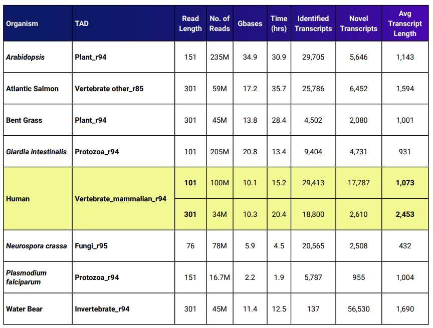
DNASTAR’s auto-annotation approach for de novo transcriptome assembly results in many identified transcripts, even for many non-model organisms. Table 1 shows benchmarks for this workflow. The assembly time needed using Lasergene Genomics version 17.3 is approximately half what was needed to assemble these sets in previous versions of SeqMan NGen.
Table 1. Benchmarks for SeqMan NGen’s de novo transcriptome assembly workflow using Lasergene Genomics 17.3.

The yellow rows show two benchmarks for human data. One data set had an average read length that was 2.98x longer compared to the other set. The average transcript length for the set with longer reads was 2.29x the average transcript length of the shorter reads.
Analyze gene expression
If you are using transcriptome data to identify differential gene expression, sifting through vast amounts of data can be cumbersome. And if you are working with a non-model organism, the lack of an available reference sequence can make this workflow extremely difficult or even impossible using typical software solutions.
But with Lasergene Genomics, gene expression analysis is easy, no matter which organism you are studying. After performing the de novo transcriptome assembly described above, there are just two additional steps.
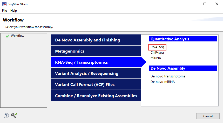
First, use SeqMan NGen to follow the templated RNA-Seq assembly workflow (Figure 8).

Figure 8. The location of the templated RNA-Seq workflow on SeqMan NGen’s “Workflow” screen.
When prompted to add sample sequences, upload the same data set you used to create the de novo transcriptome assembly. When prompted to add a reference sequence, click Add Folder and upload the .fasta output from the de novo transcriptome assembly. You can choose to use the fully-annotated identified transcripts, novel transcripts, or both (Figure 9).

Figure 9. Specifying which transcripts to use as references in the RNA-Seq assembly.
If you exported a subset of transcripts during analysis in SeqMan Ultra, you can alternatively use those by clicking Add and adding the exported .fas file.
Second, open the results in ArrayStar to quantify the relative abundances of the transcripts used in this project and analyze gene expression. Following the steps above means that the gene names associated with the transcripts can be displayed automatically in ArrayStar. ArrayStar’s advanced filtering tools, robust statistical analyses, and rich, graphical views that allow you to effortlessly isolate gene sets of interest and identify their biological significance and ontology.
In the example below, transcriptome data from a non-model organism is used to identify upregulated genes in an experiment. First, the gene table was sorted by its log2 fold change column so that the upregulated genes in the “induced” experiment appeared at the top of the table. The boxes next to the eleven most upregulated genes were then checked, causing them to appear as white dots in the associated scatterplot (Figure 10). These genes could be saved as a set for additional analysis.

Figure 10. ArrayStar’s scatter plot after selecting the most upregulated genes (in white) in an “induced” experiment.

